End to end crater analysis
This examples illustrates how to to analyze a crater surface with craterslab. We will use this xyz file with a three dimensional cloud point from the lunar crater King.
- The example is structured as follows:
Note
You can access the script of this example.
1. Setup dependencies
Import all the dependencies:
from craterslab.sensors import DepthMap, SensorResolution
from craterslab.visuals import plot_2D, plot_3D, plot_profile
from craterslab.craters import Surface
2. Loading Data
Since the data is in the form of a cloud point, we need to convert it into a depth map. To do so, we have to map those points into a matrix whose values represent the z value from the points and the indices i,j from the matrix will be proportional to their x and y coordinates respectively. So, the x coordinate form the points will be determined by i * M while the y coordinate will equal j * N, where M and N are the spacial resolution of the depth map on each axis respectively.
In craterslab, we can define the desired resolution of the depth map by:
data_resolution = SensorResolution(235.65, 235.65, 1.0, "m")
where the last parameters establishes the scale in which all computations will be made. Then, the first two parameters define M and N respectively, and can be thought of as the number of units in real scale (meters in this case) between two consecutive pixels from the depth map. The third parameter accounts from the scale in the z axis (how many sensor units equal one real scale unit).
Then, we can use this resolution to create a DepthMap as:
depth_map = DepthMap.from_xyz_file("king.xyz", resolution=data_resolution)
depth_map.crop_borders(ratio=0.25)
The last line is optional and it is only meant to remove the borders from the depth map since those do not contain information from the crater in this particular case.
Finally, we can create a Surface using a depth map. Surfaces in craterslab are a higher abstraction meant to discern important information from the depth maps.
s = Surface(depth_map)
A surface object allows for the classification of eventual craters found in the depth map. Then, for surfaces classified as craters or sand mounds, it is possible to compute an elliptical model that fits the surface, estimates the largest profile across the surface and compute some of its observables. An overview of the analysis conducted over the depth map can be inspected by simply printing the surface object:
print(s)

"""
Found: Simple crater

Apparent Depth (d_max): -2280.23 m
Eccentricity (epsilon): 0.13
Diameter (D): 78188.58 m
Maximum heigh (H_cp): 3063.19 m
Mean Heigh over the rim (mean_h_rim): 1350.90 m
Concavity Volume (V_in): 5392654283113.74 m³
Excavated Volume (V_ex): 4729292363304.89 m³
Excess Volume (V_exc): 4664067973505.89 m³
"""
3. Plotting
We can produce different plots from the depth map in order to visualize every detail of it. First, we could consider a two dimensional plot where we can optionally include the elliptical model and the largest profile:
plot_2D(depth_map, profile=s.max_profile, ellipse=s.em)

Then, we can produce a similar plot in three dimensions, where we can even scale every axis independently in order to emphasize any desired surface characteristic:
plot_3D(depth_map, preview_scale=(1, 1, 5))

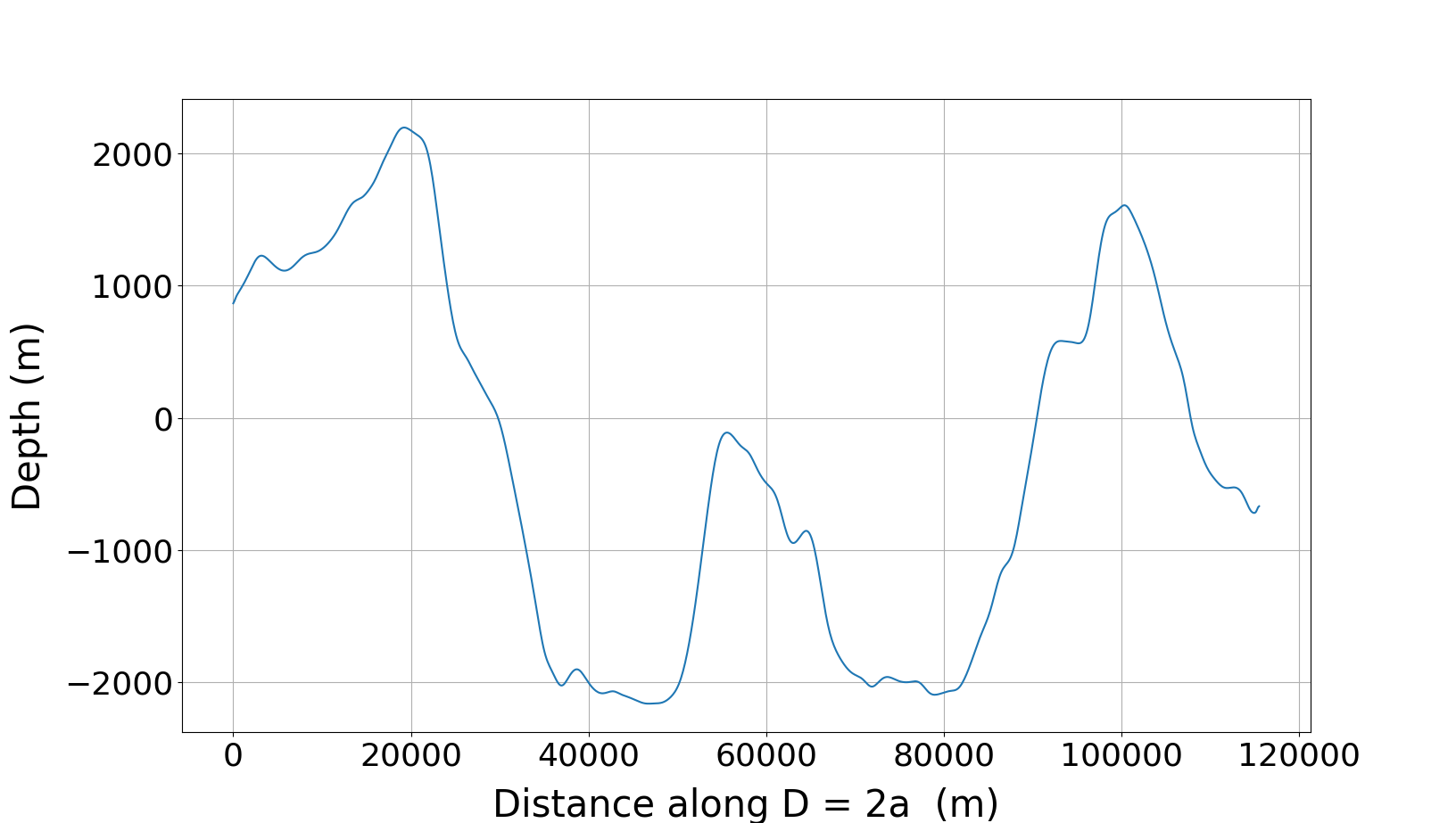
Finally, we can visualize the largest profile from the surface by:
plot_profile(s.max_profile, block=True)