Visualization tools

DepthMap objects can be inspected through different visualizations. In this example we are going to cover the available tools from craterslab that enable a visual inspection of the data.

For all the plots shown we will be using this depth map, which can be directly loaded with craterslab as:

from craterslab.sensors import DepthMap
depth_map = DepthMap.load("fluidized_1.npz")
depth_map.auto_crop()

Two-dimensional plots

In order to visualize the depth map in 2 dimensions as an image, the third dimension is encoded as the visual intensity of each pixel. In craterslab we can get this kind of visualization as:

from craterslab.visuals import plot_2D
plot_2D(depth_map, block=True)

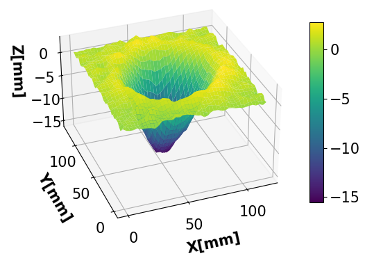
Three-dimensional plots

Similarly, we can produce a Three-dimensional plot with:

from craterslab.visuals import plot_3D
plot_3D(depth_map, block=True)

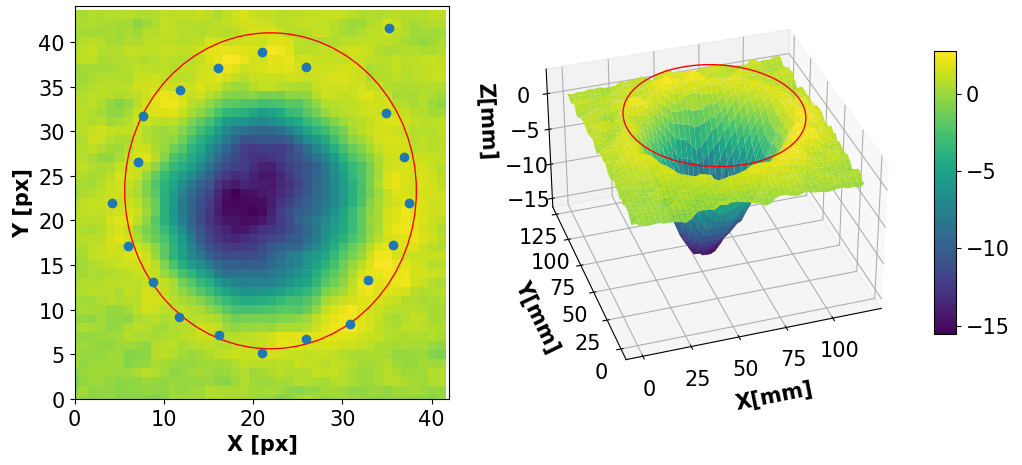
Elliptical models

For those depth maps that contain craters, it is often useful to find an elliptical model that fits the crater rims. To do so, craterslab searches for k different points evenly spaced along the crater rims. Then, those points are used to fit an ellipse. The following code snippet illustrates how to compute an elliptical model for a depth map using 20 points:

from craterslab.ellipse import EllipticalModel
em = EllipticalModel(depth_map, 20)

Now, we can include this model into the 2D and 3D plots shown before by simply passing the model as an optional argument:

from craterslab.visuals import plot_2D, plot_3D
plot_2D(depth_map, ellipse=em)
plot_3D(depth_map, ellipse=em, block=True)

That will show the computed ellipse in both plots, resulting in:

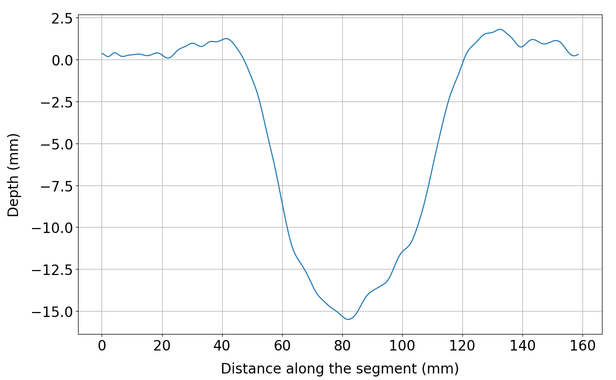
Profile plots

Besides visualizing the whole depth map, it may be wanted to visualize a certain profile of it. In other words, ‘cut’ the depth map across a segment and see how the third dimension varies along the segment. To extract a profile from a depth map in craterslab, we only need to specify the start and end points from the segment:

from craterslab.profiles import Profile
p = Profile(depth_map, (0,0), (40,40))

Then, we can inspect the profile by:

from craterslab.visuals import plot_profile
plot_profile(p, block=True)

That will show the computed ellipse in both plots, resulting in:

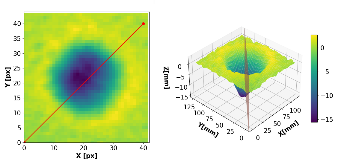
As we just did with the the ellipse, we can include a reference to a profile in the two- and three-dimensional plots:

from craterslab.visuals import plot_2D, plot_3D
plot_2D(depth_map, profile=p)
plot_3D(depth_map, profile=p, block=True)